Divine Tips About How Do I Create A Filter Table In Excel
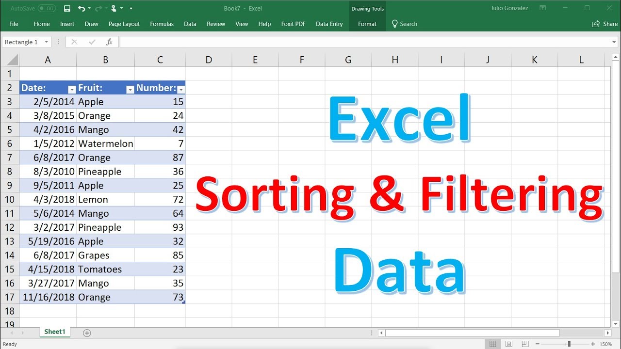
Excel Sorting And Filtering Data Youtube
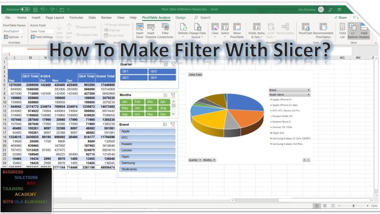
How To Make Filter By Using Slicer Pivot Table Excel? Youtube

How To Filter A Table Based On Another In Excel
How To Create Filter In Excel Youtube
How To Create Filter In Excel
Filter your excel data to only display records that meet certain criteria.
Mastering Filter Tables in Excel: A Guide to Streamlined Data Analysis
In the realm of data manipulation, Microsoft Excel remains an indispensable tool. Among its myriad functionalities, the ability to create and utilize filter tables stands out as a crucial skill for anyone aiming to extract meaningful insights from large datasets. Imagine sifting through a mountain of information, searching for that one specific detail. Without filters, it's akin to finding a needle in a haystack. But with a well-constructed filter table, this daunting task transforms into a swift, precise operation. Let's delve into the process of creating and effectively using filter tables in Excel, ensuring your data analysis is both efficient and accurate.
The essence of a filter table lies in its capacity to selectively display data based on predefined criteria. This allows users to focus on relevant information, thereby simplifying complex datasets. Whether you're analyzing sales figures, inventory levels, or survey responses, filter tables provide a dynamic way to explore and understand your data. Moreover, this functionality is not just about filtering; it's about transforming raw data into actionable intelligence. By mastering filter tables, you empower yourself to make informed decisions swiftly and confidently.
Consider the scenario of a marketing analyst tasked with evaluating the performance of various advertising campaigns. Without filters, comparing campaign results across different demographics or time periods would be a tedious, error-prone endeavor. However, with filter tables, the analyst can quickly isolate and compare specific campaign segments, identifying trends and optimizing strategies. This capability not only saves time but also enhances the accuracy of the analysis, leading to more effective marketing outcomes. And, yes, it helps avoid the dreaded 'spreadsheet-induced headache'.
The beauty of Excel's filter functionality is its user-friendly interface. Even those with limited technical expertise can quickly grasp the basics and begin applying filters to their data. This accessibility democratizes data analysis, enabling a wider audience to leverage the power of Excel for their specific needs. So, let’s get started with the how-to, shall we?
Step-by-Step Guide to Creating a Filter Table
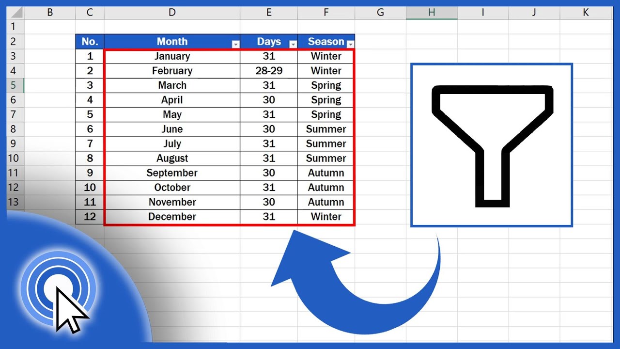
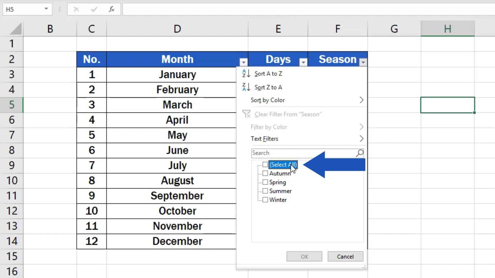
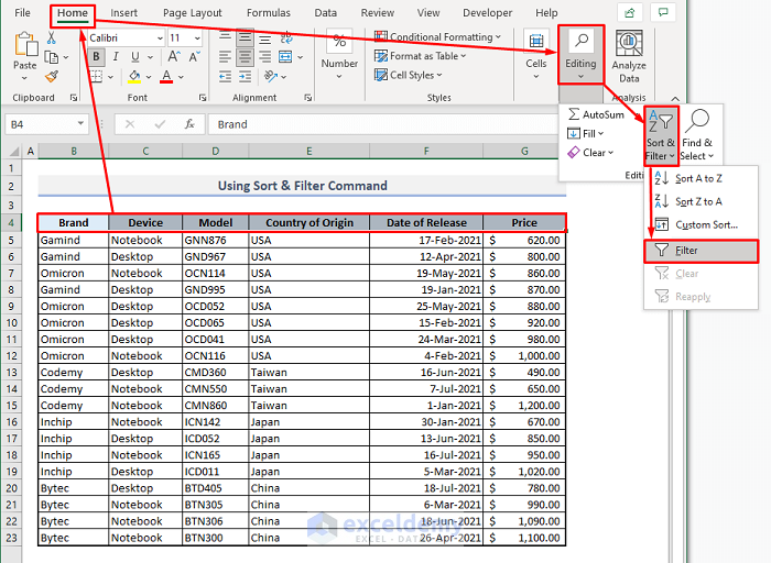
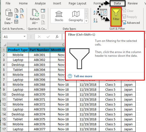
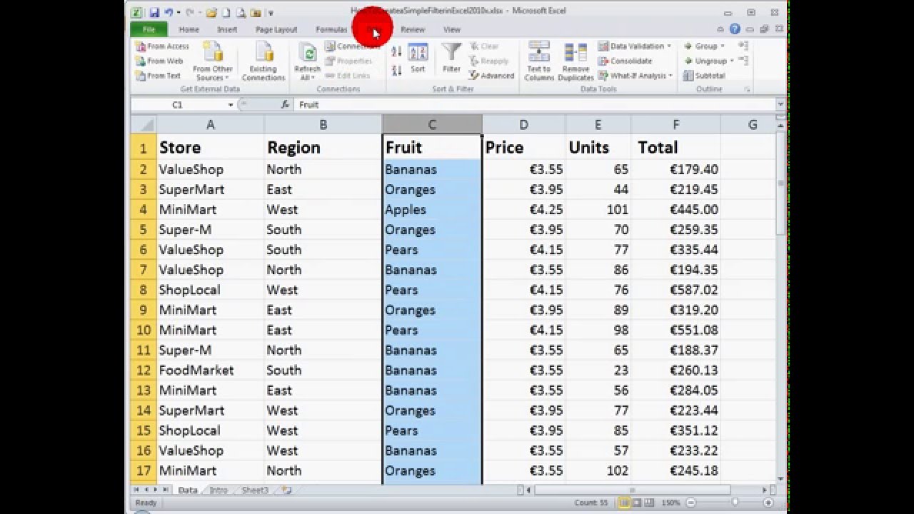
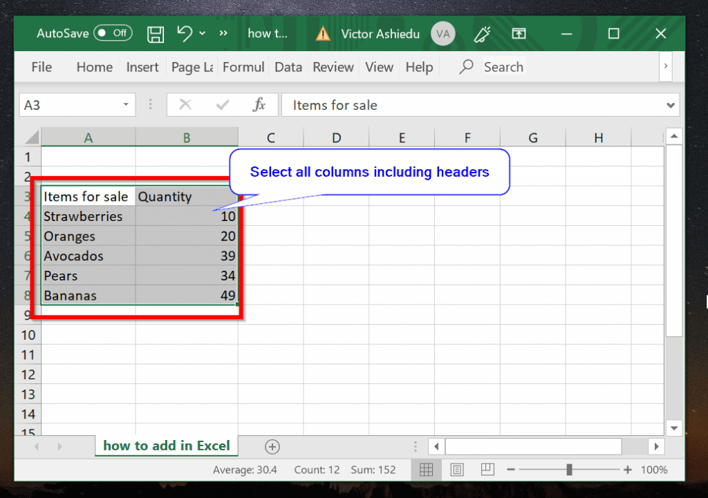
The first step in creating a filter table is to ensure your data is organized in a tabular format, with clear headers for each column. Select the range of cells that contain your data, including the headers. Once selected, navigate to the "Data" tab on the Excel ribbon. Within the "Sort & Filter" group, you'll find the "Filter" button. Click it, and voilà! Small dropdown arrows will appear in each column header, indicating that filters have been applied.
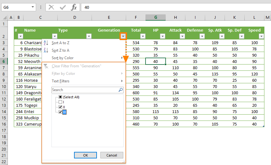
Now, let's explore how to use these filters. Click on the dropdown arrow in the column you wish to filter. A menu will appear, displaying various filtering options. You can choose to filter by specific values, text, numbers, or dates, depending on the data type in the column. For instance, if you're filtering a column containing product categories, you can select specific categories to display, hiding the rest. You can also use text filters to find items containing specific keywords, or number filters to find values within a certain range. It's like having a digital detective at your fingertips.
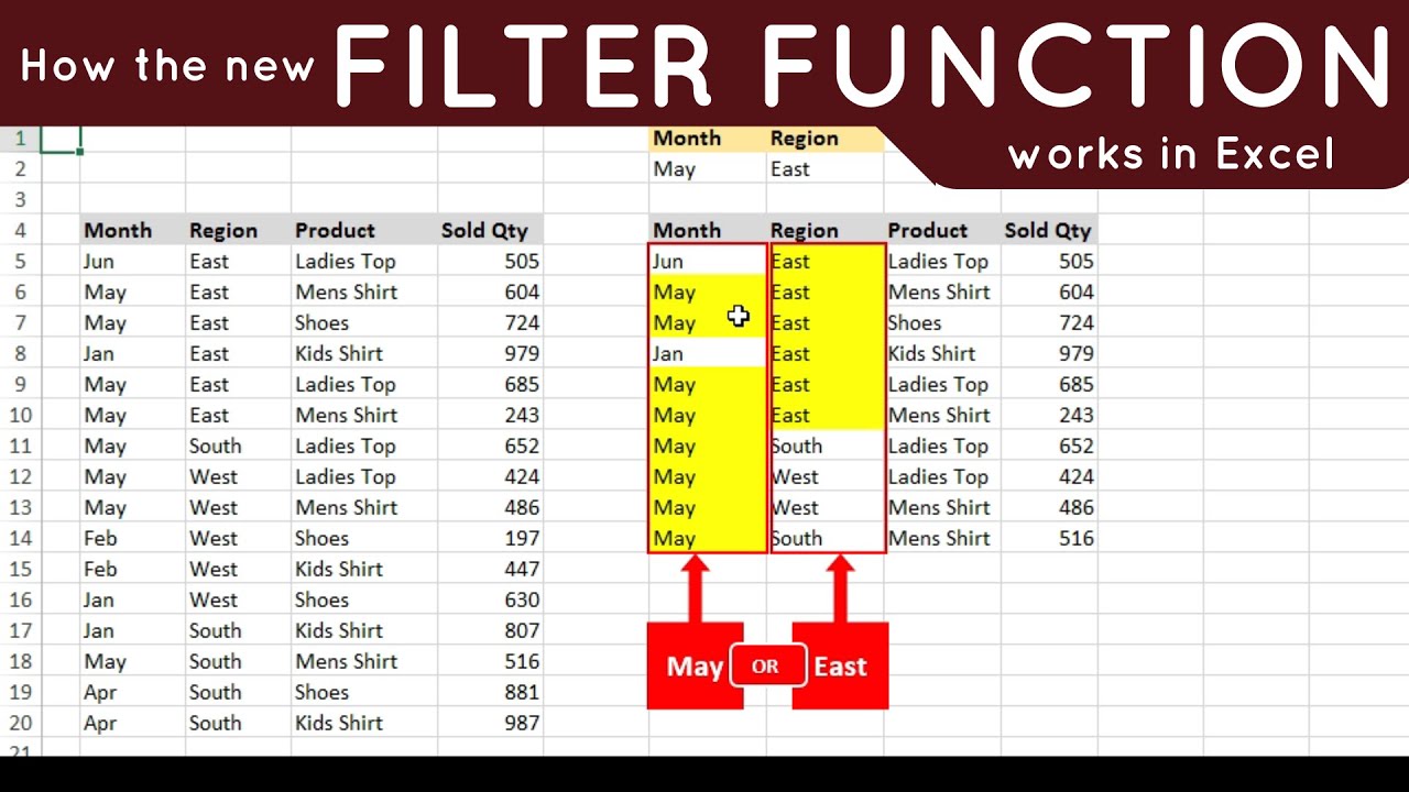
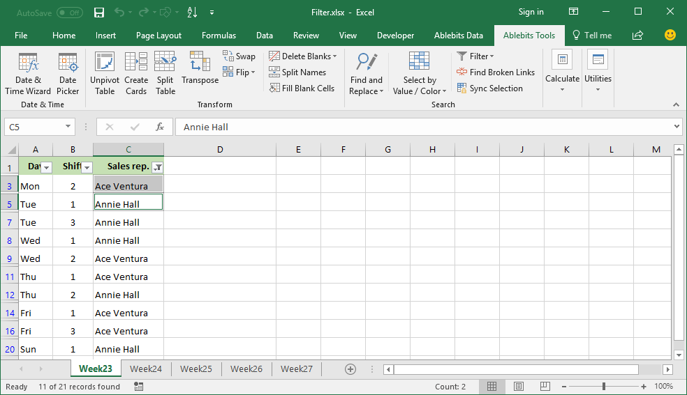
One of the most powerful features of filter tables is the ability to apply multiple filters simultaneously. You can filter data across several columns, narrowing down your results to a very specific subset. For example, you might want to see all sales transactions for a particular product category in a specific region during a certain time period. By applying filters to the product, region, and date columns, you can quickly achieve this level of granularity. This layered filtering approach allows you to uncover intricate patterns and relationships within your data.
And remember, if you make a mistake, or want to start afresh, you can easily clear the filters by going back to the "Data" tab and clicking the "Clear" button within the "Sort & Filter" group. This will remove all applied filters, restoring your data to its original state. Don't worry, Excel won't hold it against you.
Advanced Filtering Techniques
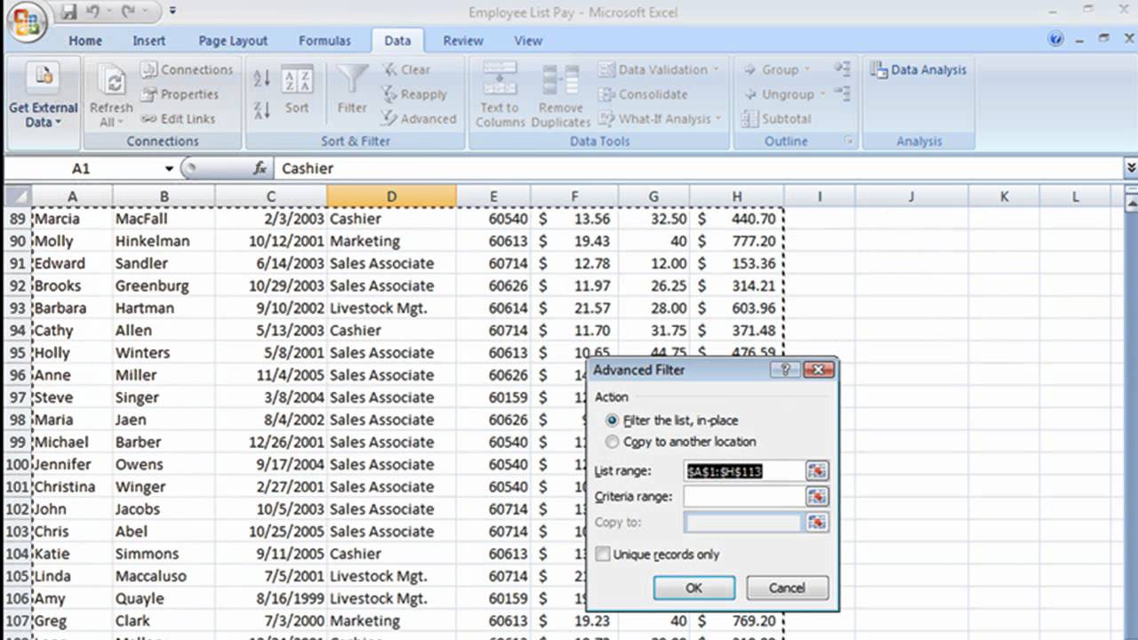
Beyond basic filtering, Excel offers advanced filtering options that provide even greater control over your data. Custom filters allow you to define more complex criteria, such as filtering for values that are greater than a certain number and less than another. This is particularly useful when dealing with numerical data where you need to identify values within a specific range. It's like setting up a digital bouncer for your data, only allowing specific entries to pass.
Another powerful feature is the ability to filter by color. If you've formatted your data using conditional formatting or manual color coding, you can filter based on cell color, font color, or icon sets. This allows you to quickly identify and analyze data points that share a common visual attribute. For example, you might color-code cells based on performance metrics, making it easy to filter and focus on high-performing or low-performing items.
For those dealing with text data, Excel provides advanced text filters that allow you to search for patterns using wildcard characters. The asterisk (*) wildcard represents any sequence of characters, while the question mark (?) wildcard represents any single character. This enables you to perform more flexible and powerful text searches. For instance, you can use the wildcard "A*" to find all items that start with the letter "A," or "*xyz*" to find all items that contain the sequence "xyz."
And, of course, don’t forget that you can also sort the filtered data! Once you've applied your filters, you can further refine your results by sorting the displayed data based on one or more columns. This allows you to arrange your data in a specific order, making it easier to identify trends and patterns. Sorting and filtering together, they are the dynamic duo of data analysis!
Optimizing Filter Tables for Large Datasets
When working with large datasets, optimizing the performance of your filter tables becomes crucial. Excel can sometimes slow down when filtering massive amounts of data, but there are several strategies you can employ to mitigate this issue. First, ensure that your data is well-organized and formatted consistently. Inconsistent data formatting can lead to slower filtering and inaccurate results. It's like trying to find a matching pair of socks in a disorganized drawer – it takes longer than it should.
Another effective strategy is to convert your data range into an Excel table. Tables offer several performance advantages over regular data ranges, including improved filtering speed and automatic expansion when you add new data. To convert your data range into a table, select the range and press Ctrl+T. This will open the "Create Table" dialog box. Ensure that the "My table has headers" option is checked, and click "OK."
Consider using indexed columns for frequently filtered data. Indexing can significantly improve filtering speed, especially for large datasets. To index a column, you can use Excel's built-in table features or create custom indexes using formulas. However, indexing can increase the file size, so use it judiciously. It's a trade-off between speed and storage, like choosing between a sports car and a minivan.
Finally, periodically review and clean your data to remove any unnecessary or redundant information. This can help reduce the size of your dataset and improve filtering performance. Regular maintenance is essential for keeping your Excel files running smoothly, just like regular oil changes for your car.
Troubleshooting Common Filter Table Issues
Even with careful planning and execution, you may encounter issues when working with filter tables. One common problem is that filters may not display all the expected values. This can occur if your data contains hidden rows or columns, or if the data range is not correctly defined. Always double-check your data range and ensure that all rows and columns are visible.
Another issue is that filters may not work correctly with merged cells. Merged cells can interfere with Excel's filtering functionality, leading to unexpected results. It's generally best to avoid merged cells in data ranges that you plan to filter. If you must use merged cells, consider creating a separate copy of your data for filtering purposes. It's like having a backup plan for your data analysis.
Sometimes, filters may not work correctly with data that contains leading or trailing spaces. These spaces can cause Excel to treat seemingly identical values as different, leading to incorrect filtering results. Use Excel's TRIM function to remove any leading or trailing spaces from your data. It's a small step that can make a big difference in the accuracy of your filters.
And if all else fails, remember the golden rule of IT: have you tried turning it off and on again? Closing and reopening Excel can sometimes resolve unexpected issues. It's the digital equivalent of a deep breath and a fresh start.
FAQ: Filter Tables in Excel
Q: How do I filter for blank cells in Excel?
A: When you click the filter dropdown, you'll see an option labeled "(Blanks)". Select this to display only the rows with blank cells in that column.
Q: Can I save a filtered view of my data?
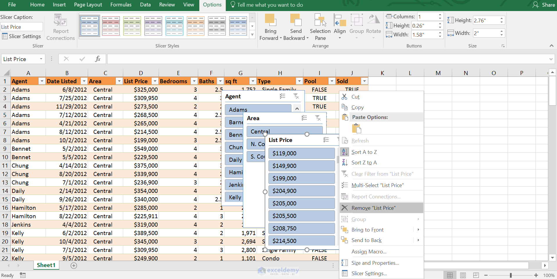
A: Yes, you can copy the filtered data and paste it into a new worksheet. Alternatively, you can create an Excel table and use Slicers to create interactive filter views that can be saved.
Q: How do I filter for dates within a specific range?
A: Click the filter dropdown for
How To Filter Multiple Rows In Excel 11 Suitable Methods Exceldemy

Excel Tutorial How To Filter A Pivot Table Globally
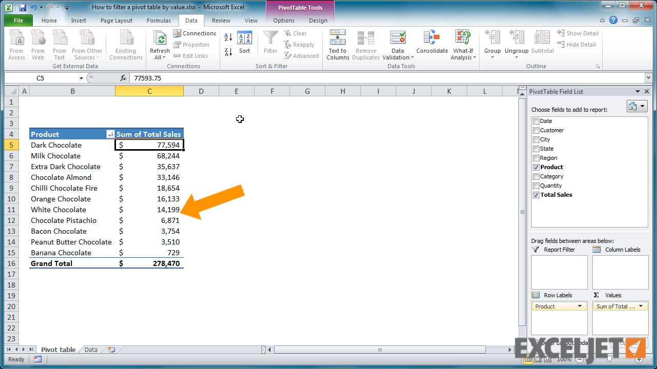
Excel Tutorial How To Filter A Pivot Table By Value

How To Make Data Tables In Excel 60 Seconds Envato Tuts+

Tutorial Filtering In Excel Tables With Video Pdf Printable Ebook 51090
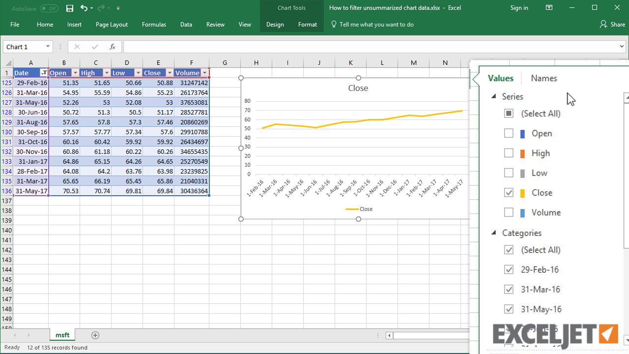
Excel Tutorial How To Filter Chart Data With A Table

How To Add Filter Labels In Excel At John Wells Blog
How To Filter An Excel Spreadsheet Slay Unty1998
How To Create A Filter For Pivot Table In Excel Printable Online
How To Use Slicers Filter A Table In Excel 2013
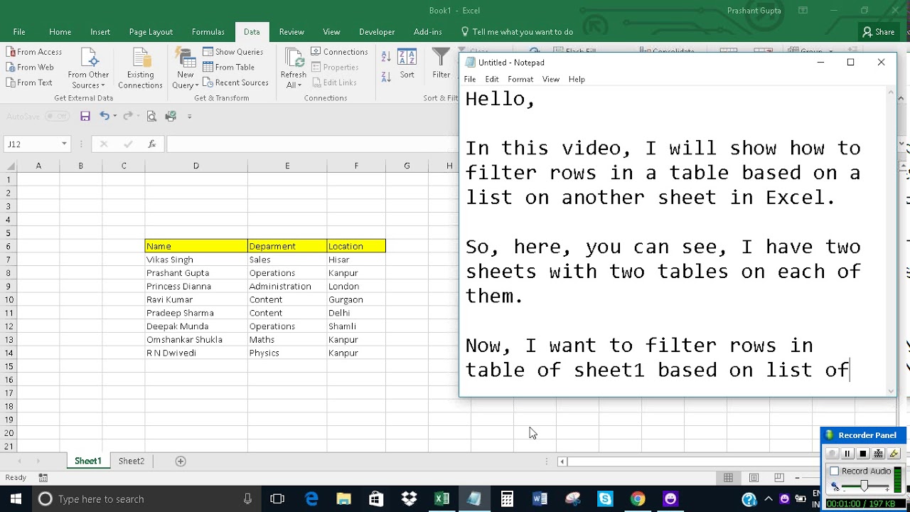
Filter Rows In A Table Based On List Another Sheet Excel Youtube

How To Use Sort And Filter With Excel Table Exceldemy
Create Custom Filters Using Excel Advanced Filter Youtube
:max_bytes(150000):strip_icc()/FilterOptions-5bdb307cc9e77c00518380f3.jpg)
How A Filter Works In Excel Spreadsheets
How To Add A Filter In Excel Printable Templates Your Goto Resource
How To Sum A Filtered Column In Excel Printable Templates
Excel Filter Table Based On Cell Value, By Multiple Values
How To Add An Auto Filter A Table In Excel. Mindovermetal English
